Jason Amey Mini Project 01

Fiscal Characteristics of Major US Public Transit Systems

Public transit in the United States serves a critical role in urban mobility. Serving millions of commuters while reducing congestion, pollution, and reliance on personal vehicles, transit is a critical institution in the success of the United States.

However there exists a wide variation in the fiscal efficiency of these systems. Understanding these financial dimensions is essential for evaluating both the sustainability and performance of transit services.

This report explores data from major U.S. public transit systems, with analysis focused on factors such as: fare revenue per mile, vehicle revenue miles (VRM), unlinked passenger trips (UPT), and the ratio of expenses to fare-box recovery.

The data thus provides insights into important components of tranist analysis including: which systems operate most efficiently, which modes of transport generate the most revenue, and how these metrics differ throughout the United States.

Using tools from the R programming language, we explore these trends over time along with the influence of population density, geography, and mode-type on a transit system’s financial outcomes. Through this exploration, we hope to better understand the complex relationship among transit usage, financial sustainability, and regional transit characteristics.

Data Creation :

if(!require("tidyverse")) install.packages("tidyverse")
library(tidyverse)

if(!require("DT")) install.packages("DT")
library(DT)

if(!require("stringr")) install.packages("stringr")
library(stringr)

if(!require("lubridate")) install.packages("lubridate")
library(lubridate)

FARES <- readxl::read_xlsx("data/mp-01/2022_fare_revenue.xlsx") |>
  select(-`State/Parent NTD ID`,
         -`Reporter Type`,
         -`Reporting Module`,
         -`TOS`,
         -`Passenger Paid Fares`,
         -`Organization Paid Fares`) |>
  filter(`Expense Type` == "Funds Earned During Period") |>
  select(-`Expense Type`)

EXPENSES <- readr::read_csv("data/mp-01/2022_expenses.csv") |>
  select(`NTD ID`,
         `Agency`,
         `Total`,
         `Mode`) |>
  mutate(`NTD ID` = as.integer(`NTD ID`)) |>
  rename(Expenses = Total) |>
  group_by(`NTD ID`, `Mode`) |>
  summarize(Expenses = sum(Expenses)) |>
  ungroup()

TRIPS <- readxl::read_xlsx("data/mp-01/2022_ridership.xlsx", sheet="UPT") |>
  filter(`Mode/Type of Service Status` == "Active") |>
  select(-`Legacy NTD ID`,
         -`Reporter Type`,
         -`Mode/Type of Service Status`,
         -`UACE CD`,
         -`TOS`) |>
  pivot_longer(-c(`NTD ID`:`3 Mode`),
               names_to="month",
               values_to="UPT") |>
  drop_na() |>
  mutate(month=my(month)) # Parse _m_onth _y_ear date specs

MILES <- readxl::read_xlsx("data/mp-01/2022_ridership.xlsx", sheet="VRM") |>
  filter(`Mode/Type of Service Status` == "Active") |>
  select(-`Legacy NTD ID`,
         -`Reporter Type`,
         -`Mode/Type of Service Status`,
         -`UACE CD`,
         -`TOS`) |>
  pivot_longer(-c(`NTD ID`:`3 Mode`),
               names_to="month",
               values_to="VRM") |>
  drop_na() |>
  group_by(`NTD ID`, `Agency`, `UZA Name`,
           `Mode`, `3 Mode`, month) |>
  summarize(VRM = sum(VRM)) |>
  ungroup() |>
  mutate(month=my(month)) # Parse _m_onth _y_ear date specs

USAGE <- inner_join(TRIPS, MILES) |>
  mutate(`NTD ID` = as.integer(`NTD ID`))

FINANCIALS <- inner_join(FARES, EXPENSES, join_by(`NTD ID`, `Mode`))

FINANCIALS <- FINANCIALS |>
  rename(
         "mode" = "Mode"
  )

FINANCIALS <- FINANCIALS |>
  mutate(mode=case_when(
    mode == "HR" ~ "Heavy Rail",
    mode == "DR" ~ "Demand Response",
    mode == "FB" ~ "Ferry Boat",
    mode == "MB" ~ "Motor Bus",
    mode == "SR" ~ "Streetcar",
    mode == "TB" ~ "Trolleybus",
    mode == "VP" ~ "Vanpool",
    mode == "CB" ~ "Commuter Bus",
    mode == "RB" ~ "Bus Rapid Transit",
    mode == "LR" ~ "Light Rail",
    mode == "YR" ~ "Hybrid Rail",
    mode == "MG" ~ "Guided Transit (Monorail)",
    mode == "CR" ~ "Commuter Rail",
    mode == "AR" ~ "Alaska Railroad",
    mode == "TR" ~ "Tramway",
    mode == "HR" ~ "Heavy Rail",
    mode == "IP" ~ "Inclined Plane",
    mode == "PB" ~ "Publico",
    mode == "CC" ~ "Cable Car",
    TRUE ~ "Unknown"))

TASK 1 - Creating Syntactic Names

Renaming column UZA Name to metro_area:

USAGE <- USAGE |>
  rename("metro_area" = "UZA Name",
         "unlinked_passenge_trips" = "UPT",
         "vehicle_revenue_miles" = "VRM",
         "agency" = "Agency",
         "mode" = "Mode"
        ) |>
  select(-"3 Mode")

output:

Data for King County Transit

NTD ID	agency	metro_area	mode	month	unlinked_passenger_trips	vehicle_revenue_miles
1	King County	Seattle–Tacoma, WA	DR	2002-01-01	135,144	746,158
1	King County	Seattle–Tacoma, WA	DR	2002-02-01	127,378	656,324
1	King County	Seattle–Tacoma, WA	DR	2002-03-01	136,030	726,578
1	King County	Seattle–Tacoma, WA	DR	2002-04-01	142,204	736,975
1	King County	Seattle–Tacoma, WA	DR	2002-05-01	144,697	746,158
1	King County	Seattle–Tacoma, WA	DR	2002-06-01	131,833	696,633

---

TASK 2 - Recoding the Mode Column

Expanding DOT mode codes into their full definitions All of the code definitions are found here: National Transit Database NTD Glossary

USAGE <- USAGE |>
  mutate(mode=case_when(
    mode == "HR" ~ "Heavy Rail",
    mode == "DR" ~ "Demand Response",
    mode == "FB" ~ "Ferry Boat",
    mode == "MB" ~ "Motor Bus",
    mode == "SR" ~ "Streetcar",
    mode == "TB" ~ "Trolleybus",
    mode == "VP" ~ "Vanpool",
    mode == "CB" ~ "Commuter Bus",
    mode == "RB" ~ "Bus Rapid Transit",
    mode == "LR" ~ "Light Rail",
    mode == "YR" ~ "Hybrid Rail",
    mode == "MG" ~ "Guided Transit (Monorail)",
    mode == "CR" ~ "Commuter Rail",
    mode == "AR" ~ "Alaska Railroad",
    mode == "TR" ~ "Tramway",
    mode == "IP" ~ "Inclined Plane",
    mode == "PB" ~ "Publico",
    mode == "CC" ~ "Cable Car",
    TRUE ~ "Unknown"))

sample_n(USAGE, 20) |>
  select(agency, metro_area, mode)

output:

Data for Full Definition Transit Modes

agency	metro_area	mode
Birmingham-Jefferson County Transit Authority	Birmingham, AL	Motor Bus
Yolo County Transportation District	Sacramento, CA	Motor Bus
Michiana Area Council of Governments	Elkhart, IN–MI	Motor Bus
Lower Rio Grande Valley Development Council	McAllen, TX	Demand Response
Potomac and Rappahannock Transportation Commission	Washington–Arlington, DC–VA–MD	Demand Response
Greater Richmond Transit Company	Richmond, VA	Vanpool
Stanislaus Regional Transit Authority	Modesto, CA	Demand Response
Worcester Regional Transit Authority	Worcester, MA–CT	Demand Response
Chattanooga Area Regional Transportation Authority	Chattanooga, TN–GA	Motor Bus
Knoxville-Knox County Community Action Committee	Knoxville, TN	Demand Response
Pinellas Suncoast Transit Authority	Tampa–St. Petersburg, FL	Bus Rapid Transit
Laketran	Cleveland, OH	Commuter Bus
METRO Regional Transit Authority	Akron, OH	Motor Bus
Regional Transportation Commission of Washoe County	Reno, NV–CA	Demand Response
Kanawha Valley Regional Transportation Authority	Charleston, WV	Motor Bus
Maryland Transit Administration	Baltimore, MD	Light Rail
Transit Joint Powers Authority for Merced County	Merced, CA	Demand Response
Broward County Board of County Commissioners	Miami–Fort Lauderdale, FL	Motor Bus
Regional Transportation Program, Inc.	Portland, ME	Demand Response
Central Midlands Regional Transportation Authority	Columbia, SC	Commuter Bus

---

TASK 3 - Answering Instructor Specified Questions with dplyr

Using functions we have studied in class, including filter, group_by, summarize, arrange, answer the following questions in your analysis:

Question 1

What transit agency had the most total VRM in this sample?

USAGE |>
  filter(!is.na(agency)) |>
  group_by(agency) |>
  summarize(total = sum(vehicle_revenue_miles)) |>
  arrange(desc(total))

output:

Data for Agency with Largest Vehicle Revenue Miles

agency	total
MTA New York City Transit	10,832,855,350
New Jersey Transit Corporation	5,645,525,525
Los Angeles County Metropolitan Transportation Authority	4,354,016,659
Washington Metropolitan Area Transit Authority	2,821,950,701
Chicago Transit Authority	2,806,202,144

Answer 1

MTA New York City Transit: 10,832,855,350 Vehicle Revenue Miles

Note:

New York City is the largest city in the United States and the “big city” with the highest percentage of its residents using mass transit. These findings are in line with the signature characteristics of NYC’s transportation demographics.

---

Question 2

What transit mode had the most total VRM in this sample?

USAGE |>
  filter(!is.na(mode)) |>
  group_by(mode) |>
  summarize(total_vrm = sum(vehicle_revenue_miles, na.rm = TRUE)) |>
  arrange(desc(total_vrm))

output:

Data for Mode with Largest Vehicle Revenue Miles

mode	total_vrm
Motor Bus	49,444,494,088
Demand Response	17,955,073,508
Heavy Rail	14,620,362,107
Commuter Rail	6,970,644,241
Vanpool	3,015,783,362

Answer 2

Motor Bus: 49,444,494,088 Vehicle Revenue Miles

Note:

Outside a few major eastern US cities, much of the United States transportation infrastructure is meant to serve motorized vehicles. It is logical then that the motor bus would far outnumber the miles traveled by rail and other forms of transit.

---

Question 3

How many trips were taken on the NYC Subway (Heavy Rail) in May 2024?

USAGE |>
  filter(
    month =="2004-05-01" &
    mode == "Heavy Rail" &
    agency == "MTA New York City Transit"
  ) |>
  select(agency, mode, month, unlinked_passenge_trips)

output:

Data for Trips Taken on NYC Subway in May 2024

agency	mode	month	unlinked_passenger_trips
MTA New York City Transit	Heavy Rail	2004-05-01	184,334,430

Answer 3

184,334,430 trips

If you divide this figure by 30 (days in a month), and then divide that result by 8,300,000 (population of NYC), the average New Yorker takes .7402 subway rides a day.

---

~~Question 4

What mode of transport had the longest average trip in May 2024?

---

Question 5

How much did NYC subway ridership fall between April 2019 and April 2020?

 subway_ridership <- USAGE |>
  filter(
      agency == 'MTA New York City Transit' &
      mode == "Heavy Rail" &
      (month == "2019-05-01" | month == "2020-05-01")
      )

subway_ridership_2019 <- subway_ridership[1,]$unlinked_passenge_trips
subway_ridership_2020 <- subway_ridership[2,]$unlinked_passenge_trips

subway_ridership_2019 - subway_ridership_2020

# [1] 210561702

Answer 5

184,334,430

Note:

Covid sucked.

---

Three (four) more interesting transit facts in this data

FACT 1

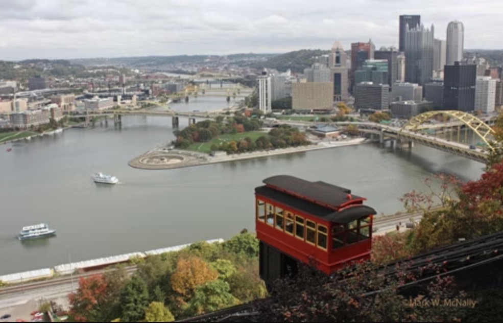
In Pittsburgh, PA there is a unique form of uphill rail transit called the Duquesne Incline. It offers arguably the most scenic view of Downtown Pittsburgh and the convergence of the city’s “Three Rivers.” Do tourists largely ride the Duquesne Incline? :

from Wikipedia:

The incline was intended to carry cargo up and down Mt. Washington in the late 19th century. It later carried passengers, particularly Mt. Washington residents who were tired of walking up the steep footpaths to the top of the bluff. Inclines were being built all over Mt. Washington to serve working-class people who were forced out of the lowlying riverfront by industrial development

I was interested to see if the ridership numbers suggested any traditional transit usage, or if the incline was now primarily used for “transit tourism”.

month_map <- c(
  "01" = "January",
  "02" = "February",
  "03" = "March",
  "04" = "April",
  "05" = "May",
  "06" = "June",
  "07" = "July",
  "08" = "August",
  "09" = "September",
  "10" = "October",
  "11" = "November",
  "12" = "December"
)

USAGE |>
  filter(startsWith(agency, "Pitt")) |>
  filter(mode == "Inclined Plane") |>
  mutate(month_split = strsplit(as.character(month), "-")) |>
  mutate(month_num = sapply(month_split, function(x) x[2])) |>
  mutate(month_name = month_map[month_num]) |>
  group_by(month_name) |>
  summarize(total_this_month = sum(unlinked_passenge_trips)) |>
  arrange(desc(total_this_month))

output:

Data for Yearly Ridership of the Pittsburgh Inclined Plane

month_name	total_this_month
July	1,715,940
August	1,507,425
June	1,424,861
May	1,224,003
September	1,128,166
October	1,061,274
April	1,032,881
November	965,257
March	895,805
December	877,248
January	666,924
February	641,834

Conclusion

The ridership numbers spiking in the summer, along with stark drop off in ridership from December to January, suggest the incline is largely popular with tourists and not used as much by the hill-weary residents of Mt. Washington.

---

FACT 2

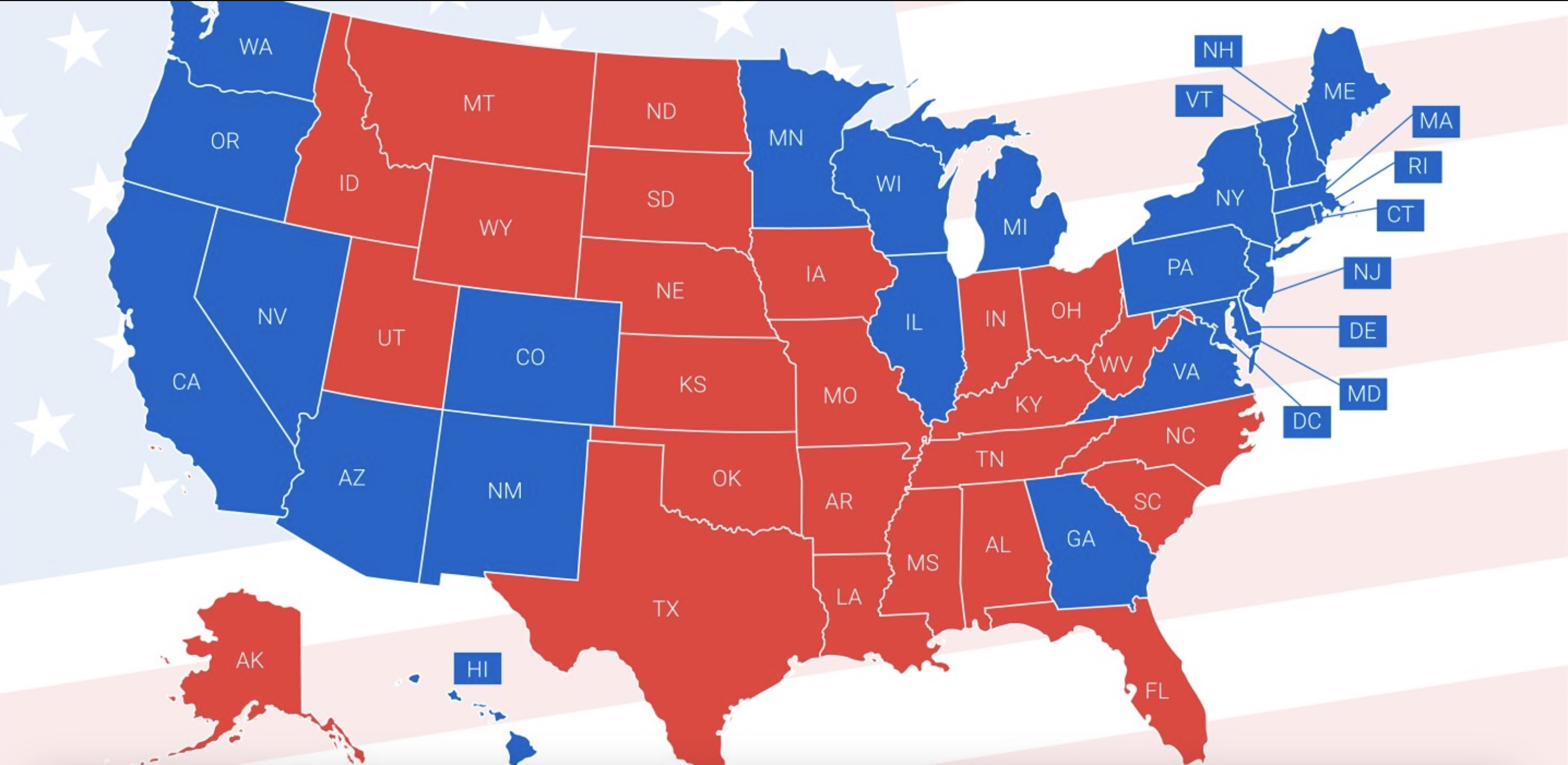
As our country remains polarized on so many issues and cultural concern, I was curious if there was an obvious Red vs. Blue divide over transit usage in this country.

I wanted to see if I could identify any obvious distinctions or division in the use of transit between Red States and Blue States.

USAGE |>
  #there is def some code smell here :
  mutate(state_split = strsplit(metro_area, ", ")) |>
  mutate(state = sapply(state_split, function(st) st[2])) |>
  mutate(state_split = strsplit(state, "-")) |>
  mutate(state = sapply(state_split, function(st) st[1])) |>
  group_by(state) |>
  summarize(total_trips = sum(unlinked_passenge_trips)) |>
  arrange(desc(total_trips)) |>
  print(n = 20)

output:

Data for Total State Transit Trips

state	total_trips
NY	85,530,025,008
CA	27,099,834,336
IL	12,744,773,889
DC	9,057,818,580
PA	8,776,976,555
MA	7,993,427,892
FL	5,742,223,542
TX	5,466,164,685
WA	4,524,992,934
GA	3,096,203,662
OR	2,555,837,796
OH	2,364,107,111
MD	2,271,510,025
CO	2,144,454,426
MN	1,909,216,918
MI	1,776,345,495
NV	1,395,503,197
AZ	1,384,679,690
MO	1,371,031,013
HI	1,225,521,578

Conclusion

There does in fact look to be a Red vs. Blue divide over transit usage in this country. While this list is indeed dominated by many Blue States, I believe the most convincing evidence for this fact are state rankings #7 - #11.

Both Florida, Texas and Georgia - all Red States - are among the largest states by population in the United States.

1. Florida Population: 22.4 million
2. Texas Population: 30.03 million
3. Georgia Population: 10.9 million

However, Oregon and Washingon are neighbors to those 3 large Red states in this ranking of transit use.

Yet Oregon and Washington - both Blue States - are medium-sized states in terms of population counts.

1. Washington Population 7.786 million
2. Oregon Population 4.2 million

That Oregon and Washinton maintain comparable volumes of transit usage, despite significantly lower populations than large Red States like Florida, Texas and Georgia, suggest there is a Red v. Blue divide over transit usage in the United States.

A better exercise would be to measure transit trips / population to see the per capita number for ridership.

---

FACT 3

This is interesting :

USAGE |>
  group_by(agency) |>
  summarize(total_trips = sum(unlinked_passenge_trips),
            total_miles = sum(vehicle_revenue_miles),
            num_ppl_mile = total_trips / total_miles
            ) |>
  arrange(desc(total_trips)) |>
  slice(1:50) |>
  arrange(desc(average_trip)) |>
  print(n = 50)

output:

agency	total_trips	total_miles	num_ppl_mile
New York City Department of Transportation	440,538,576	4,150,573	106
Washington State Ferries	502,394,973	20,230,767	24.8
City and County of San Francisco	4,533,445,698	583,200,690	7.77

Conclusion

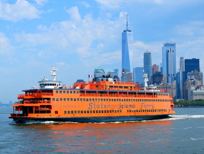
This looks to be communicating that Ferries are very efficient vehicles for transporting a lot of people over small distances. Every SI Ferry carries around ~4,000 people !

---

FACT 4

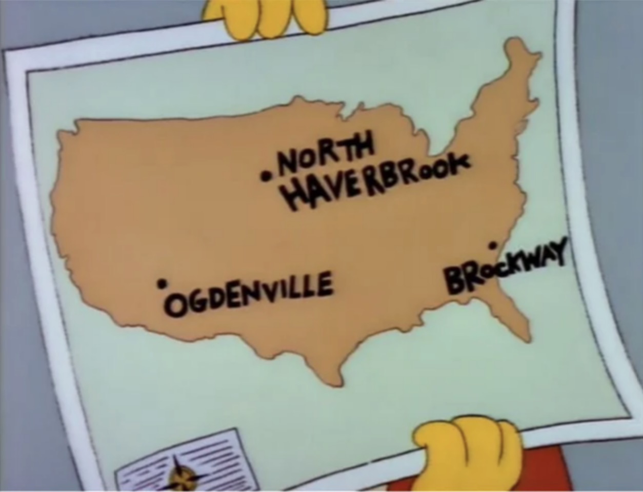
This charismatic, tune-carrying charlatan has swindled unknowing cities like Ogdenville, North Haverbrook and Brockway into buying dubious monorail systems for their communities.

I was interested to see where this snake-oil salesman - with a voice of gold! - has worked his sly sales magic across the United States…

USAGE |>
  filter(mode == "Guided Transit (Monorail)") |>
  group_by(metro_area) |>
  summarize(count = n())

output:

Monorails Systems in the United States

metro_area	count
Detroit, MI	151
Jacksonville, FL	151
Las Vegas–Henderson–Paradise, NV	34
Miami–Fort Lauderdale, FL	151
Morgantown, WV	145
San Francisco–Oakland, CA	116
Seattle–Tacoma, WA	151

Conclusion

Detroit, MI, Morgantown, WV and Jacksonville, FL are a few of the US cities where brain-dead slobs work cushy jobs on this very unique, very rare form of mass transit.

---

Task 5: Table Summarization

Create a new table from USAGE that has annual total (sum) UPT and VRM for 2022. This will require use of the group_by, summarize, and filter functions. You will also want to use the year function, to extract a year from the month column.

USAGE_2022_ANNUAL <- USAGE |>
  mutate(year = year(month)) |>
  filter(year(month) == 2022) |>
  group_by(year, metro_area, agency, mode, `NTD ID`) |>
  summarize(total_upt = sum(unlinked_passenge_trips, na.rm = TRUE),
            total_vrm = sum(vehicle_revenue_miles, na.rm = TRUE)) |>
  select(`NTD ID`, agency, metro_area, mode, total_upt, total_vrm, year) |>
  filter(total_upt > 400000) |>
  ungroup()

USAGE_AND_FINANCIALS <- left_join(USAGE_2022_ANNUAL,
                                  FINANCIALS,
                                  join_by(`NTD ID`, mode)) |>
  rename(
    "total_fares" = "Total Fares",
    "expenses" = "Expenses",
  ) |>
  select(-"Agency Name") |>
  drop_na() |>
  
print(USAGE_AND_FINANCIALS, n = 5)

output:

Data for 2022 Usage and Financials

NTD ID	agency	metro_area	mode	total_upt	total_vrm	year	total_fares	expenses
50010	METRO Regional Transit Authority	Akron, OH	Motor Bus	3,470,765	3,252,489	2022	2,345,779	38,200,740
50021	Portage Area Regional Transportation Authority	Akron, OH	Motor Bus	591,881	672,463	2022	1,933,660	6,197,595
20002	Capital District Transportation Authority	Albany–Schenectady, NY	Motor Bus	12,656,760	8,723,783	2022	7,947,384	95,586,715
60019	City of Albuquerque	Albuquerque, NM	Bus Rapid Transit	1,829,848	792,000	2022	38,268	6,535,431
60019	City of Albuquerque	Albuquerque, NM	Motor Bus	4,151,408	3,788,377	2022	738,682	40,436,564

---

Task 6: Farebox Recovery Among Major Systems

Question 1

Which transit system (agency and mode) had the most UPT in 2022?

USAGE_AND_FINANCIALS |>
  arrange(desc(total_upt)) |>
  select(agency, mode, total_upt)

output:

Transit GOATs

agency	mode	total_upt
MTA New York City Transit	Heavy Rail	1,793,073,801
MTA New York City Transit	Motor Bus	458,602,305
Los Angeles County Metropolitan Transportation Authority	Motor Bus	193,637,448
Los Angeles County Metropolitan Transportation Authority	Motor Bus	193,637,448
Chicago Transit Authority	Motor Bus	140,013,945

Answer 1

MTA New York City Transit Heavy Rail: 1,793,073,801

Note:

While New York City’s inclusion on this list is understandable, along with Chicago: the 3rd largest city in the United States, seen as an historical pre-war, pre-automobile city… the inclusion of Los Angeles County is arguably surprising.

While LA County is of significant population size, it is considered a “sprawled out” metro area most friendly to the automobile. Despite this reputation, and despite the challenges of offering transit in a region with lower population density, LA county’s high transit ridership suggests the existence of an undeniable appetite for quality transit.

---

Question 2

Which transit system (agency and mode) had the highest farebox recovery, defined as the highest ratio of Total Fares to Expenses?

USAGE_AND_FINANCIALS |>
  mutate(farebox_recovery = total_fares / expenses ) |>
  arrange(desc(farebox_recovery)) |>
  select(agency, mode, farebox_recovery) |>
  print(n = 5)

output:

Private Ride You’re Going to Pay

agency	mode	farebox_recovery
Port Imperial Ferry Corporation	Ferry Boat	1.43
Hyannis Harbor Tours, Inc.	Ferry Boat	1.41
Trans-Bridge Lines, Inc.	Commuter Bus	1.33
Chattanooga Area Regional Transportation Authority	Inclined Plane	1.31
Regional Transportation Commission of Washoe County	Vanpool	1.24

Answer 2

Port Imperial Ferry Corporation, Ferry Boat: 1.43

Note:

Port Imperial Ferry, Haynnis Harbor Tours and Trans-Bridge Lines are all private companies. As private companies, their fares must exceed their expenses as their operations are not supported by any government entity. Furthermore, business owners expect profit on their capital investment and assumption of risk. This is consistent with an observation of fares outpacing revenue.

---

Question 3

Which transit system (agency and mode) has the lowest expenses per UPT?

USAGE_AND_FINANCIALS |>
  mutate(expenses_UPT = expenses / total_upt ) |>
  arrange(expenses_UPT) |>
  select(agency, mode, expenses_UPT)

output:

Where is the NYU Shuttle?

agency	mode	expenses_UPT
North Carolina State University	Motor Bus	1.18
Anaheim Transportation Network	Motor Bus	1.28
University of Iowa	Motor Bus	1.54
Chatham Area Transit Authority	Ferry Boat	1.60
Texas State University	Motor Bus	2.05

Answer 3

North Carolina State University, Motor Bus : 1.18 $/ride

Note:

It’s logical that the transit systems with the lowest expense per ride serve universities. College campuses are communities with two factors suited for offering affordable, cost-sensitive transit: a high population density (students are mostly in dorms and shared housing) and a smaller surface for transit coverage (the routes are limited to a college campus, not an entire city).

---

Question 4

Which transit system (agency and mode) has the highest total fares per UPT?

USAGE_AND_FINANCIALS |>
  mutate(fares_UPT = total_fares / total_upt ) |>
  arrange(desc(fares_UPT)) |>
  select(agency, mode, fares_UPT)

output:

Soak the Rich

agency	mode	fares_UPT
Hampton Jitney, Inc.	Commuter Bus	41.3
Pennsylvania Department of Transportation	Commuter Rail	32.3
Hyannis Harbor Tours, Inc.	Ferry Boat	29.6
Trans-Bridge Lines, Inc.	Commuter Bus	28.1
SeaStreak, LLC	Ferry Boat	22.1

Answer 4

Hampton Jitney: 41.3 $/trip

Note:

The Hampton Jitney is a logical candidate to collect the highest fares for every ride (i.e. its riders pay the most) because it is responsible for transporting some the wealthiest residents of New York City to some of the most desirable vacationing in the United States - the famed beach community “The Hamptons.” If you can charge wealthy customers more for a service they can afford, as a business person, why wouldn’t you? What’s more, the Hampton Jitney vehicles are outfitted with amenities to comfort the wealthy riders who use the service. Seemingly the higher fares are not only going to transportation expenses, but also on-bus goodies used to appeal to a luxury audience.

---

Question 5

Which transit system (agency and mode) has the lowest expenses per VRM?

USAGE_AND_FINANCIALS |>
  mutate(expenses_VRM = expenses / total_vrm ) |>
  arrange(expenses_VRM) |>
  select(agency, mode, expenses_VRM)

output:

Vanlyfe

agency	mode	expenses_VRM
Metropolitan Transportation Commission	Vanpool	0.445
San Joaquin Council	Vanpool	0.498
San Diego Association of Governments	Vanpool	0.540
Regional Transportation Commission of Washoe County	Vanpool	0.566
Los Angeles County Metropolitan Transportation Authority	Vanpool	0.581

Answer 5

Metropolitan Transportation Commission : 0.445 $/mile

Note:

Vanpool’s efficiency stems from 1. it being easier to run a smaller van at capacity than a larger bus and 2. it being subsidized by non-road users. The highway trust fund has long been running a deficit as gas tax revenues have not kept up with the cost of highway construction and maintenance. Because vanpool can run its vehicles consistently at full capacity, and can use infrastructure that is not fully supported by road user fees, it suggests an efficient form of transit.

---

Question 6

Which transit system (agency and mode) has the highest total fares per VRM?

USAGE_AND_FINANCIALS |>
  mutate(fares_VRM = total_fares / total_vrm ) |>
  arrange(desc(fares_VRM)) |>
  select(agency, mode, fares_VRM)

output:

Expensive Boats

agency	mode	fares_VRM
Jacksonville Transportation Authority	Ferry Boat	158.0
Chattanooga Area Regional Transportation Authority	Inclined Plane	149.0
Hyannis Harbor Tours, Inc.	Ferry Boat	138.0
SeaStreak, LLC	Ferry Boat	115.0
Cape May Lewes Ferry	Ferry Boat	93.0

Answer 6

Jacksonville Transportation Authority : 158.0 $/mile

Note:

Ferries are often necessary, not because a rider needs to travel long distances, but because a body of water is serving as an insurmountable transportation barrier.

Ferries are expensive. Here in NYC, ferries operate at 10X the subsidy as a subway ride. Presumably the higher fares collected by these transit agencies are needed to cover the ferry boat’s higher expenses. With the combination of a larger numerator (the ferry fares) and a smaller denominator (miles traveled) we can understand the results found here.

---

Based on all of this, what do you believe to be the most efficient transit system in the country? (Your answer may differ depending on which form of ‘efficiency’ you care most about)

Transit use is an unmistakable social, ecological and economical good. It enhances opportunity, reduces pollution and generates wealth through efficient land use.

As such, I believe the transit agency and mode that provides the most trips is the most efficient system:

MTA New York City Transit, Heavy Rail: 1,793,073,801